The Advection-Diffusion Equation

In this numerics deep dive we look at a fundamental equation of mathematical physics: the advection-diffusion equation. This equation appears in a diverse variety of applications, including fluid flow and kinetic physics. Several properties of this equations are discussed and some examples of using Lanyon to generate proofs and simulation results are shown.

The Theory

The advection-diffusion equation is a fundamental equation that describes the transport of a scalar field: the motion of the scalar is due to advection in a velocity field, and due to diffusion. The advection velocity and the diffusion tensor can either be specified or computed from other equations.

The advection-diffusion equation, despite its apparent simplicity, forms the backbone of many other complex systems. For example, in fluid flow the density and energy of the fluid advect with the fluid velocity, leading to extremely complex mixing processes that are often chaotic.

More interestingly, if we allow the flow and diffusion to be in phase-space (a higher-dimension space that combines both the spatial and momentum coordinates) then it can describe, with appropriate choices of advection velocities and diffusion tensors, kinetic physics. For example, the motion of matter under gravity (the Boltzmann equation), the path of charged particles in electromagnetic fields (the Vlasov-Maxwell equations), and plasma turbulence in magnetic confinement devices (the gyrokinetic equations) are all described by specialized forms of advection-diffusion equations.

For the purposes of this numerics deep dive we will look at the equation written in the form

$$ \frac{\partial f}{\partial t} + \nabla\cdot(\mathbf{u} f) = \nabla\cdot(\mathbf{D}\cdot\nabla f). $$

In this equation \( \mathbf{u} \) is the advection velocity, \( \mathbf{D} \) is the diffusion tensor, and \( f(x,t) \) is the advected scalar quantity. We will assume that the advection velocity and diffusion tensor are specified as functions of space and time.

Properties of the Advection-Diffusion Equation

We will begin by deriving some important properties of this equation. One would want some or all these properties to be preserved by the numerical method we choose. A general approach to deriving properties of a large class of conservation laws is to first derive the weak form of the equation. We do this by multiplying by a smooth function \( w \) and integrating over an arbitrary volume \( \Omega \) to get, after using integration by parts,

$$ \int_\Omega w \frac{\partial f}{\partial t}\thinspace d^3\mathbf{x} + \oint_{\partial\Omega} w \mathbf{n}\cdot (\mathbf{u} f - \mathbf{D}\cdot \nabla f) \thinspace ds - \int_\Omega \nabla w \cdot (\mathbf{u} f - \mathbf{D}\cdot \nabla f)\thinspace d^3\mathbf{x} = 0. $$

In a certain sense this weak form of the equation is more fundamental than the original partial differential equation (PDE) as it involves fewer derivatives, allowing for a broader class of solutions. For example, in the absence of any diffusion the weak form permits the propagation of shocks. The ability to capture shocks is critical for many applications. Specialized shock-capturing methods have been developed for such situations, and Lanyon uses such schemes by default.

The trick to proving properties is to choose different values of the weight function \( w \). We can prove, for example, by choosing \( w = 1 \) that the total amount of “stuff” in the control volume is conserved:

$$ \frac{d}{dt} \int_\Omega f d^3\mathbf{x} + \oint_{\partial\Omega} \mathbf{n} \cdot (\mathbf{u} f - \mathbf{D}\cdot \nabla f)\thinspace ds = 0. $$

This is a conservation law, that is, it says that the total integrated quantity in the volume \( \Omega \) can only change due to flux passing through the boundary \( \partial\Omega \).

We can derive another important property in the special case in which the flow velocity is incompressible, that is, when \( \nabla\cdot \mathbf{u} = 0 \). This incompressibility condition occurs very frequently in applications. For example, in most problems in phase-space (galactic dynamics, plasma physics, low-density fluid flows) the phase-space velocity is incompressible. We choose \( w = f \), that is, the solution itself as the test function. A little vector algebra shows that

$$ \frac{d}{dt}\int_\Omega \frac{1}{2}f^2 \thinspace d^3\mathbf{x} + \oint_{\partial\Omega} \mathbf{n} \cdot (\mathbf{u} \frac{1}{2} f^2 - \mathbf{D}\cdot \nabla \frac{1}{2} f^2) \thinspace ds = -\int_\Omega (\nabla f \cdot \mathbf{D} \cdot \nabla f) \thinspace d^3\mathbf{x}. $$

This expression shows that, under the condition of incompressibility, as long as \( \nabla f \cdot \mathbf{D} \cdot \nabla f > 0\) the \( L_2 \)-norm of the solution decays monotonically. Of course, the \( L_2 \)-norm will remain conserved if there is no diffusion. This condition for decay (or conservation) is satisfied if the diffusion tensor is positive semi-definite.

The monotonic decay of the \( L_2 \)-norm is important to preserve in a numerical scheme: it ensure that the scheme remains stable.

A final important property that we can show is that if initially the scalar quantity is positive, \( f(x,0) > 0 \), then it always remains positive, \( f(x,t) > 0 \). It is very hard for a numerical scheme to ensure this property, unfortunately.

In summary, the advection-diffusion equation conserves the quantity being advected, monotonically decays the \( L_2 \)-norm of the solution when the flow is incompressible and the diffusion tensor is positive semi-definite, and maintains positivity of the solution if initial conditions are positive. In constructing good numerical scheme we need to ensure that some or all of these properties are satisfied by the discrete scheme we construct. This is not always possible, and usually a balance must be found in accuracy of the scheme and its robustness properties: in general, the more accurate a scheme the less robust it is.

The Numerics

Now that we have studied a few properties of the advection-diffusion system we wish to discretize we can switch to constructing the discrete scheme. Notice that we have a time-dependent equations with first-order time-derivatives, and first and second-order spatial derivatives, including cross-derivative terms. Hence, Lanyon must:

• Choose a computational grid or mesh that is appropriate for the problem we wish to solve. In this deep-dive Lanyon will assume simple, rectangular domains and so will use a uniform, rectangular mesh.

• Once we choose the mesh, we use a discrete approximation to the spatial derivative terms that appear in the equation. For this, one needs to carefully consider where on the mesh to compute the various quantities that appear in our equation, and from this construct a discrete derivative operator of sufficient accuracy. The discrete derivative operators will be different, for example, if we use a curvilinear mesh or a triangular mesh.

• Lanyon then needs to decide how to advance the solution in time: it will replace the time derivative with a discrete approximation and advance or march the solution forward in time using a ODE solver. We will of course need to prescribe initial conditions and apply the appropriate boundary conditions.

Each of these steps - mesh generation, constructing spatial discrete operators, and choosing a time-stepper - are complicated and impact the quality of the numerical solution Lanyon will obtain. Once it has made all these choices, executable proofs of correctness for various properties (certificates) are generated, for example using the Lean proof assistant language. Though Lanyon presently uses Lean as its default proof assistant, we intend to support other theorem-provers such as Rocq and Agda in the future. Not all properties of the continuous equations are inherited by the discrete scheme. Depending on the set of problems we wish to study, we may want to ensure some key properties of the continuous scheme are inherited by the discrete scheme.

In general, as described in The Theory section above, we will also find that there is a tradeoff between accuracy of the scheme and robustness. For example, a highly accurate scheme could violate positivity, or will develop spurious high-\( k \) modes when the spatial scales of the solution approach the grid spacing. In general, some form of regularization, for example, limiters or extra diffusion, may be needed to obtain a stable and useful solver.

For the purposes of this numerics deep-dive Lamyon will make the following choices:

• It will choose a finite-volume method for the advective term, using upwinding to determine the numerical flux at each cell interface.

• To prevent oscillations when the structures in the solution get comparable to the grid size (high-\( k \) modes) it will choose an appropriate limiter that ensures that such modes do not cause serious errors.

• For the diffusion term Lanyon will choose a properly centered finite-difference scheme: recall that there is no preferred direction in diffusion and so one should not use upwinding here. There are subtle issues when the diffusion tensor is highly anisotropic. Further, analogous to problems with high-\( k \) modes, for diffusion terms other subtleties like thermodynamic consistency of the scheme arise. We shall address these topics later.

Lanyon uses a reconstruction approach to determine surface fluxes from both the advective and diffusive terms, and a special hierarchical selection to ensure robustness. At present, it does not correct for positivity violations or thermodynamic inconsistencies in the diffusion terms.

Discontinous Galerkin Discretization

The Discontinuous Galerkin (DG) schemes form an important class of higher-order method for the solution of PDEs. The key idea in the DG scheme is to assume that the solution inside each cell can be expanded as a polynomial, and then use the PDE to derive the evolution equation for each expansion coefficient. To construct a DG scheme one first selects, in each cell, a set of $N$ test functions, $\psi_k(\mathbf{x})$, $k = 1,\ldots,N$. Multiply the advection equation by $\psi_k(\mathbf{x})$, integrate over a cell $\Omega_j$ and use integration by parts to get the DG weak-form

$$ \int_{\Omega_j} \psi_k \frac{\partial f}{\partial t}\thinspace d^3\mathbf{x} + \oint_{\partial\Omega_j} \psi_k\ \mathbf{n}\cdot (\mathbf{u} f - \mathbf{D}\cdot \nabla f) \thinspace ds - \int_{\Omega_j} \nabla \psi_k \cdot (\mathbf{u} f - \mathbf{D}\cdot \nabla f)\thinspace d^3\mathbf{x} = 0 $$

for $k=1,\ldots,N$. We next expand $f$ in basis functions. In general, the set of test and basis functions need not be the same. However, in the DG method we choose the same set, and hence write

$$ f_h(\mathbf{x},t) = \sum_k f_k(t) \psi_k(\mathbf{x}). $$

The expansion coefficients $f_k(t)$ are the unknowns. Plugging this into the DG weak-form we get

$$ \frac{d}{dt} \sum_m \int_{\Omega_j} \psi_k \psi_m \thinspace d^3\mathbf{x} f_m + \oint_{\partial\Omega_j} \psi_k\ \mathbf{n}\cdot (\mathbf{u} f_h^- - \mathbf{D}\cdot \nabla f_h^-) \thinspace ds - \sum_m \int_{\Omega_j} \nabla \psi_k \cdot (\mathbf{u} \psi_m - \mathbf{D}\cdot \nabla \psi_m) \thinspace d^3\mathbf{x} f_m = 0 $$

In this equation $f_h^-$ is the value of the expansion evaluated just inside the cell. Observe an subtle issue here: the solution $f_h$ is discontinuous across cell boundaries. Then how are we to compute the needed values of the derivatives in the surface terms? One approach is to use a recovery scheme: in this we use the expansion in the two cells connected to each face to recover a polynomial that is continuous across the cell boundary. Once this polynomial is recovered than we can takes its derivatives (as it is continuous) and use it in the surface term. Note that unlike the advection terms, there is no upwind direction for diffusion. Hence, whatever process we use to determine the derivatives at the interface must be symmetric, that is, not depend on advection velocity.

Lanyon uses orthonormal polynomials in a unit cell $I_d = [-1, 1]^d$. That is,

$$ \langle \psi_k \psi_m \rangle = \delta_{km} $$

where the angle brackets indicate integration over the hypercube $I_d$. The use of orthonormal polynomials greatly simplifies the algorithm and also dramatically cuts down on computational cost. For example, the mass matrix $\langle \psi_k \psi_m \rangle$ diagonalizes, resulting in a set of uncoupled equations for each of the expansion coefficients $f_m$. Further, a large number of terms in the volume integral also drop out. With care, one can also eliminate or reduce aliasing errors, leading to an alias-free, matrix- and quadrature-free DG scheme. Details about this are described in our paper, where we also show that our modal scheme scales sub-quadratically with the number of basis functions.

The Proofs

The complete sequence of steps to run Lanyon is described below. As part of the code generation process Lanyon produces formal proofs (e.g. in Lean) to check the correctness of various properties of the solvers it builds. Example proofs for the 1D, 2D and 3D advection-diffusion equations, and the generated C code, are available on the Lanyon GitHub repo.

As we describe in detail on GitHub, Lanyon takes less than ten minutes to generate all the Lean and C code, including for DG schemes. It creates more than 20,000 lines of Lean and nearly 18,000 lines of C code. The Lean code proves the correctness of our algorithms, and Lanyon will refuse to generate C if the /verify step (see below) fails. Some examples of the Lean definitions and theorems are listed below.

• Example Definition: Lanyon generates the definition of the eigenvalues of the flux Jacobians. These eigenvalues need to be real. See the definition of hyperbolic PDEs in the Lanyon Formulary. For the advection equations the eigenvalues are simply the components of the flow velocity.

• Example Theorem: Lanyon generates a theorem that shows that the $x$-direction advective flux is hyperbolic. In the same way, Lanyon will generate proofs that the $y$- and $z$-direction advective fluxes are also hyperbolic.

• Other examples of theorems are those that show consistency of the diffusive flux in each direction, that the flux-jump relations (see) are satisfied in the $x$-direction. Many other theorems and definitions are provided, and one should consult the GitHub repo for more details.

When using the DG scheme Lanyon also generates the specification of the basis functions to use and the various surface expansion polynomials. As an example, the specification for $p=2$ DG for the advection equation is on our Github repo. Once the specification is generated we can check for properties of the basis. First, the same checks are performed as for the FV scheme to ensure hyperbolicity and the flux-jump condition, for example. Specifically for the DG scheme we check consistence of the left and right reconstructions (that is, to ensure that the volume expansions evaluated at the surface are identical to the surface expansion that Lanyon generates). We also check that the basis functions can represent exactly the polynomials of lower or equal order. The complete set of Lean4 proofs for the $p=2$ DG scheme are on our Github page.

The Results: Second-Order Methods

In this section we show a sequence of results for the advection-diffusion equation sytem in 1D and 2D. For each problem set we also give the prompts that we used in Lanyon to generate the code and simulation. In general, to construct a solver one needs to run three steps. These are:

• Step 1: Run the /specify command (see examples) to tell Lanyon what equation system you wish to solve, in which dimension. You can also add other details as desired. For more complex equation systems you may have to run the /deepthought command. An example of a generated DSL specification can be viewed on our Github repo.

• Step 2: Once Lanyon completes the specify step you should ensure that the generated specification is syntactically correct by running the /verify command. This command takes no parameters. If the /verify command fails then you may need to rerun the /specify command with some variation, or use the /deepthought command. Lanyon will refuse to build the actual simulation code if /verify does not pass.

• Step 3 Once /verify passes, then you must run the /compile command. This takes no options and will produce the C code for the solver you specified in the /specify command. Examples of generated C kernels are on our Github.

Once these steps are completed, you then run the /simulate command, describing in detail the specific simulation you want to run. Many examples are given below.

1D Advection-Diffusion

For the first test we will build a 1D advection-diffusion solver. The prompt to Lanyon is:

/specify Create a 1D advection-diffusion solver

Note the simplicity of the prompt: you do not need to specify the scheme, the limiter or any other parameters. Lanyon will choose appropriate defaults for you. At this point you will see some messages fly by, with a Lisp DSL fragment that describes the system of equatiosn. Run /verify to ensure this fragment is syntactically correct. Note that the /verify step does not check if the equation or proofs of correctness are semantically correct¹. Semantic correctness is ensured by our sophisticated RAG pipeline that embodies deep knowledge of physics and applied mathematics. This meta-level checking is, in general, not 100% foolproof as Lanyon has no way to know (especially in complex situations) what exactly the user had in mind. Such capabilities remain an active area of research for us.

Now, we are ready to run our first simulation! This is the problem of advecting two periods of a sine wave: the initial condition is $\sin(x)$ on a periodic domain, with an advection speed of $1.0$ and a constant diffusion coefficient of $0.01$.

/simulate Simulate the advection of two periods of a sin wave with advection velocity 1 and diffusion coefficient 0.01. Use 32 cells on a periodic domain.

That’s it! Lanyon now will create the simulation based on the verified C code and run it for you, producing a large amount of output, including diagnostics.

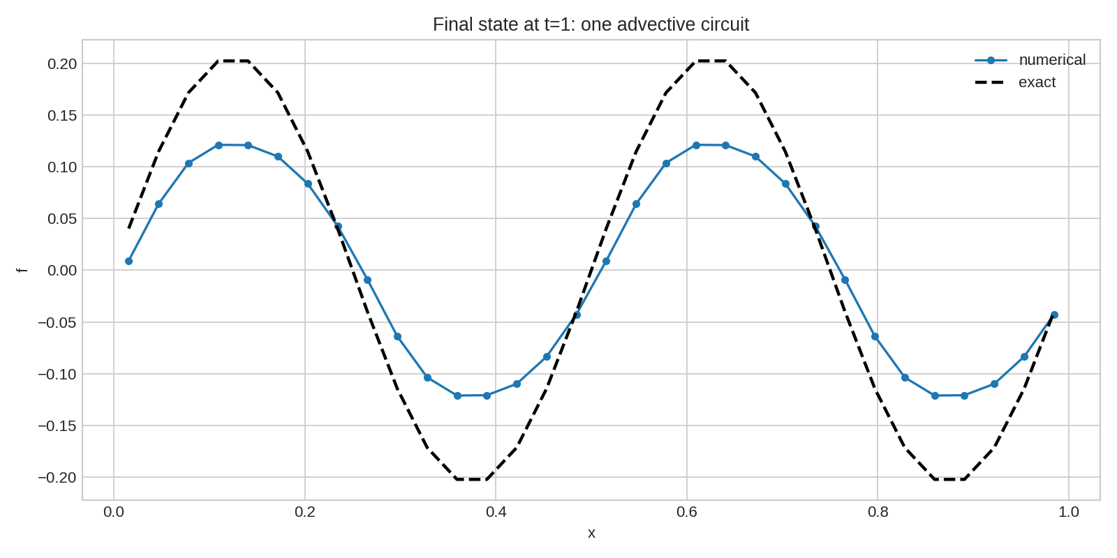
In the figure above the blue line is the solution computed by Lanyon: the scheme it chose here uses limiters and is run at a smaller CFL number, leading to some excessive numerical damping. The extra flattening of the tops of the waves is due to the limiters: use of higher-order methods with maxima/minima-preserving limiters will eliminate this issue, and we will explore this later in the Research Note.

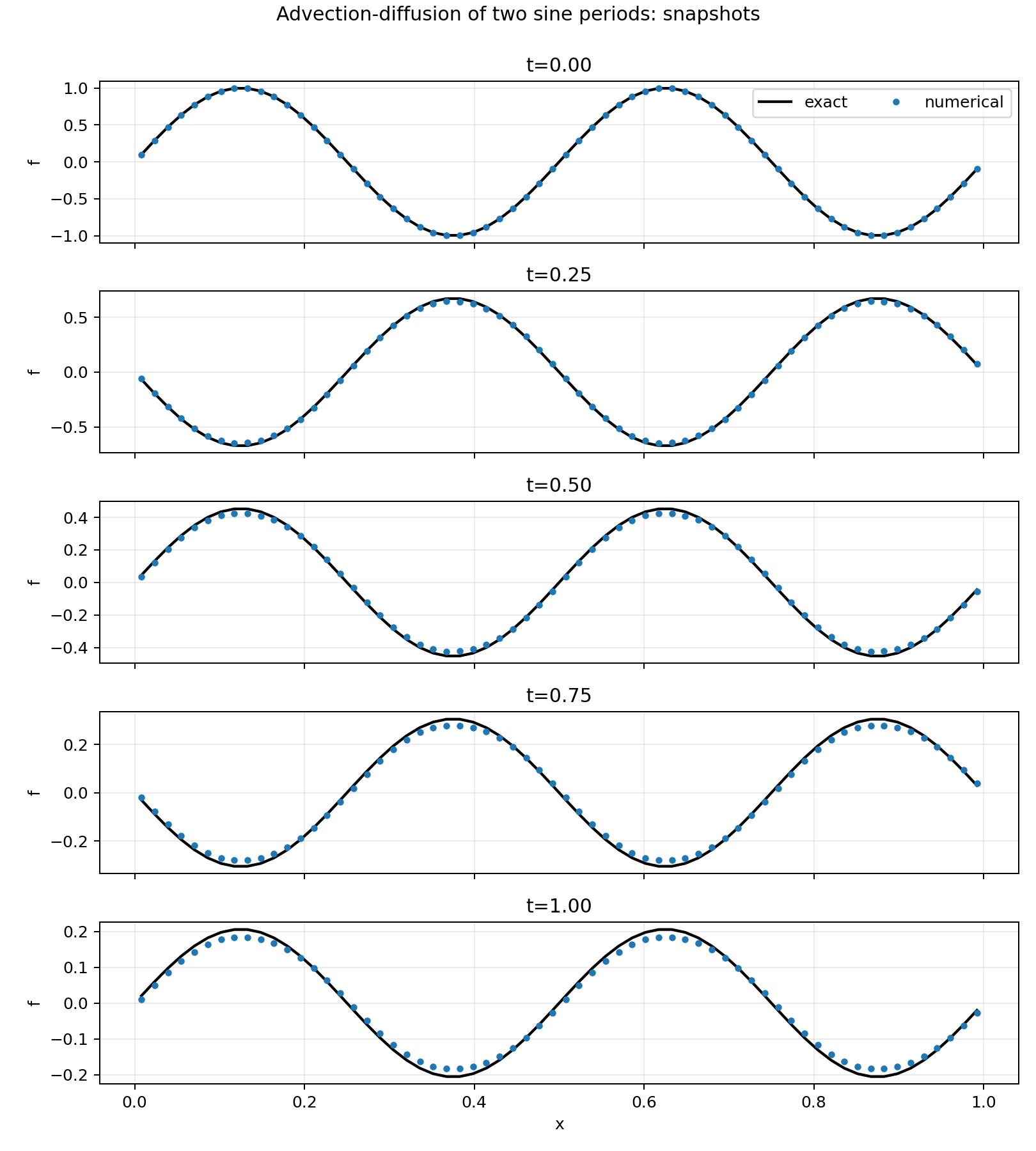
However, we can run the same simulation on a finer grid:

/simulate Simulate the advection of two periods of a sin wave with advection velocity 1 and diffusion coefficient 0.01. Use 64 cells on a periodic domain.

With this higher resolution we now get a far less numerically damped solution as seen in the following figure

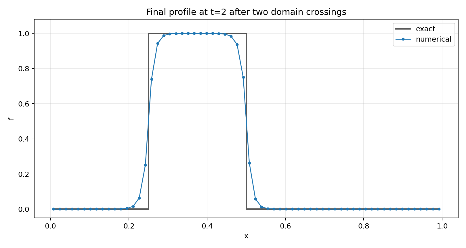
As a final test in 1D we will advect a square flat-top profile twice across a periodic domain:

/simulate Simulate the advection of a square flat-top, with unit height on a periodic domain. Set the diffusion to 0.0. Use 64 cells on a periodic domain.

This simulation checks the efficacy of the limiters (in this case the default min-mod limiter).

2D Advection-Diffusion

For this set of problems we will create a 2D advection-diffusion solver using the following simple prompt:

/specify Create a 2D advection-diffusion solver

Once the solver is created and we have run /verify and /compile, we can run simulations. The first simulation we shall run is the advection of a “cosine hump” in a rigid-body rotating flow. This flow has flow-velocity given by

$$ \begin{align} u_x &= -y+1/2 \\ u_y &= x-1/2. \end{align} $$

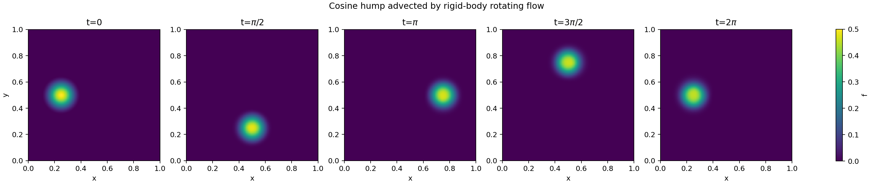
This represents a counter-clockwise rigid body rotation about $(x_c,y_c)=(1/2,1/2)$ with period $2\pi$. Hence, structures will perform a circular motion about $(x_c,y_c)$, returning to their original position at $t=2\pi$. We will choose the initial condition:

$$ f(x,y,0) = \frac{1}{4} \left[ 1 + \cos(\pi r) \right] $$

where

$$ r(x,y) = \min(\sqrt{(x-x_0)^2 + (y-y_0)^2}, r_0)/r_0 $$

The prompt we will give Lanyon is

/simulate Simulate 2D advection in a flow with x-velocity -y+1/2 and y-velocity x-1/2 on a domain that is unit length in each direction. Set diffusion to zero. Run till time of 2 pi. Use a “cosine hump” initial condition as described in https://ammar-hakim.org/sj/je/je12/je12-poisson-bracket.html#rigid-body-rotating-flow

Note a few features of this prompt: we are telling Lanyon the advection speed to use and pointing it to another webpage (or a paper) for the specific form of the initial conditions to use. The RAG pipeline will ensure the advection speed is correctly set and will attempt to use the initial conditions from the specified webpage.

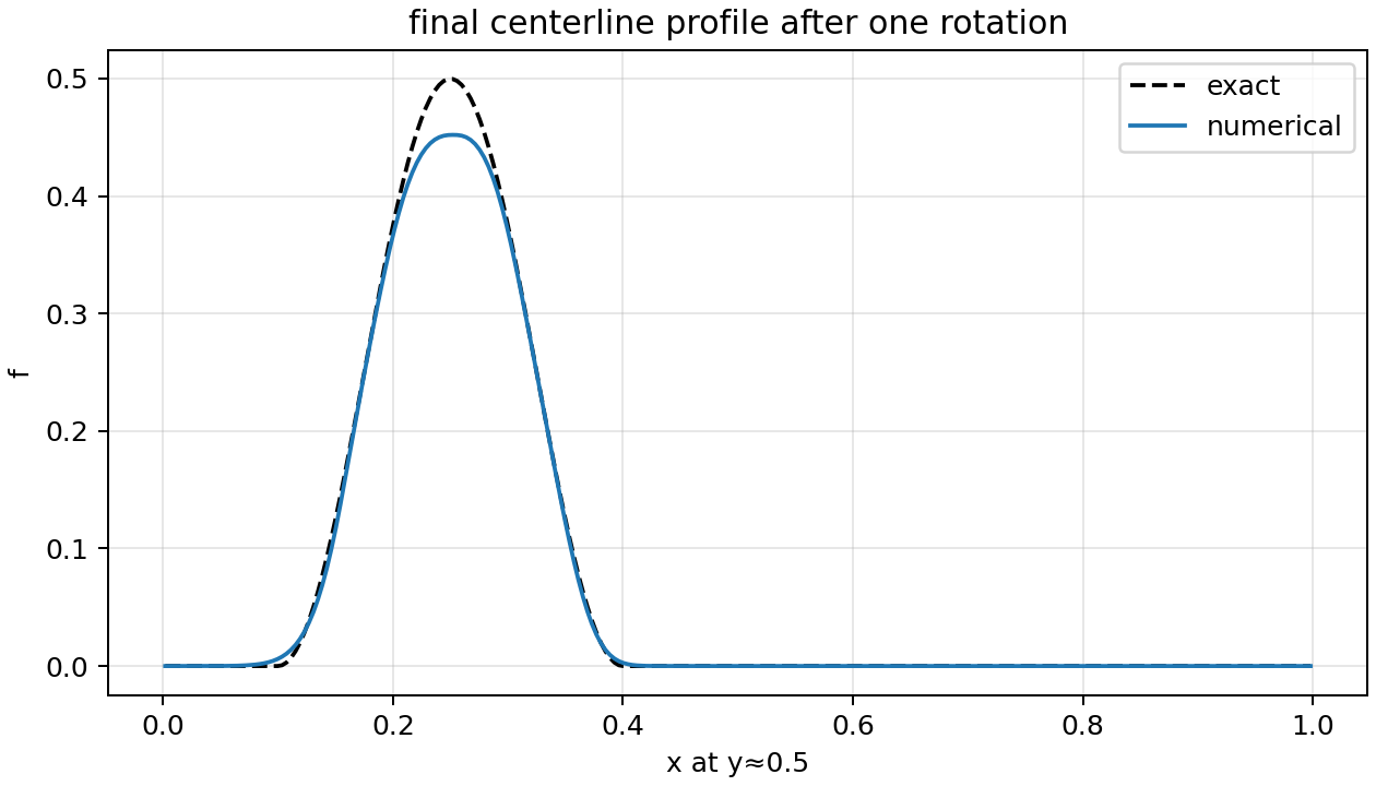
The figures below show snapshots of the solutions and a lineout of the final and the exact solutions. Note that the limiter leads to some flattening of the maxima of the “cosine hump”.

We now illustrate the ability to specify an anisotropic diffusion coefficient using the following prompt to the simulate command:

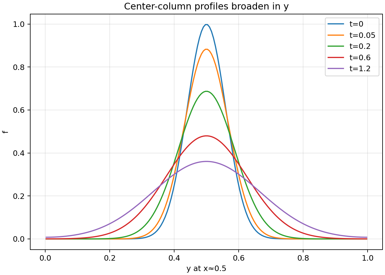
/simulate Simulate 2D diffusion only along the Y-direction. Set advection velocity to zero. Start with a Gaussian initial condition in the center of a domain and use periodic boundary conditions.

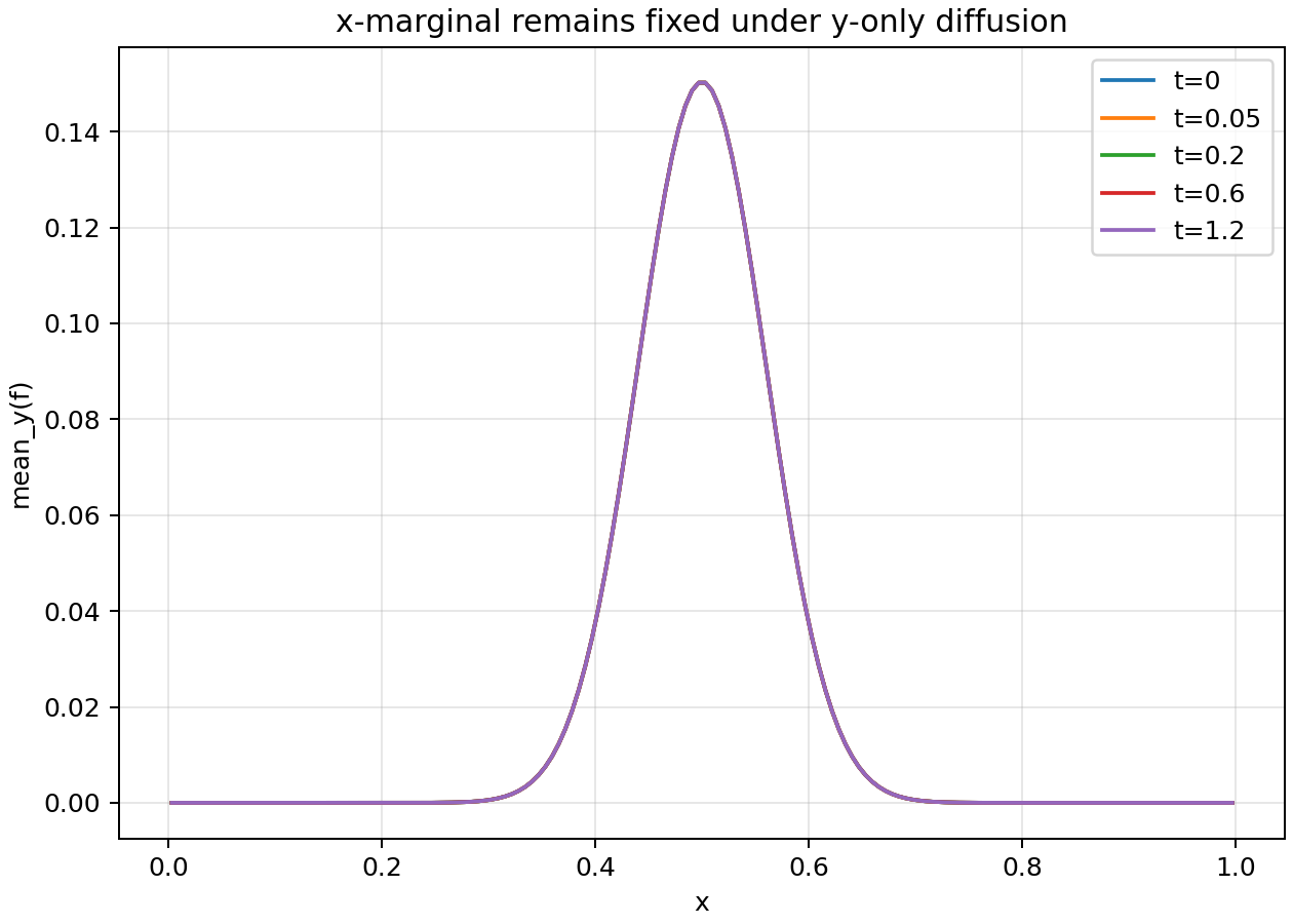
This prompt will set a default diffusion coefficent in $y$-direction, and set the diffusion in $x$-direction to zero. The figures below show the lineout in the $y$- and $x$-directions. The anisotropic diffusion causes the Gaussian to diffuse only the $y$-direction, leaving the $x$-direction shape completely unchanged.

The Results: Discontinuous Galerkin Methods

In this series of tests we create an advection equation solver using the discontinuous Galerkin scheme. First, we will create a DG scheme using polynomial order 1 basis functions:

/deepthought Create a 1D advection solver using a polynomial order 1 Discontinuous Galerkin scheme

Lanyon produces the scheme specification in a few seconds. We can then verify and compile the specification into Lean and C code, preparing for simulations.

The first simulation is to propagate a Gaussian on a periodic domain for two periods:

/simulate Simulate the advection of a Guassian with advection velocity 1 on a periodic domain for two periods. Use 32 cells.

Lanyon will now create the simulation driver and run the simulation inside a container. Snapshots of the solution at different times are shown below.

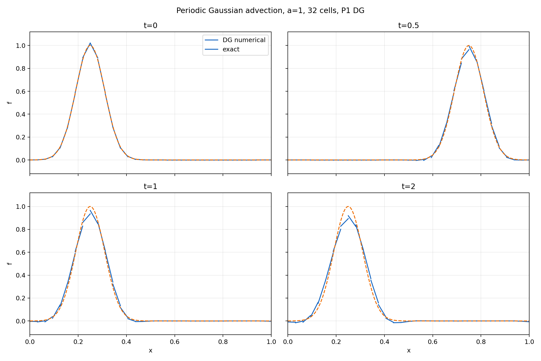
In the above figure we plot the DG solution, which are straight lines in each cell as we are using $p=1$ basis functions, at different times. The scheme shows some numerical diffusion and some dispersion, however, much less than the corresponding FV scheme at the same resolution. We can reduce the diffusion and dispersion by using $p=2$ basis functions:

/deepthought Create a 1D advection solver using a polynomial order 2 Discontinuous Galerkin scheme

We run this simulation again on the same grid. The figure below shows the snapshots of the solution:

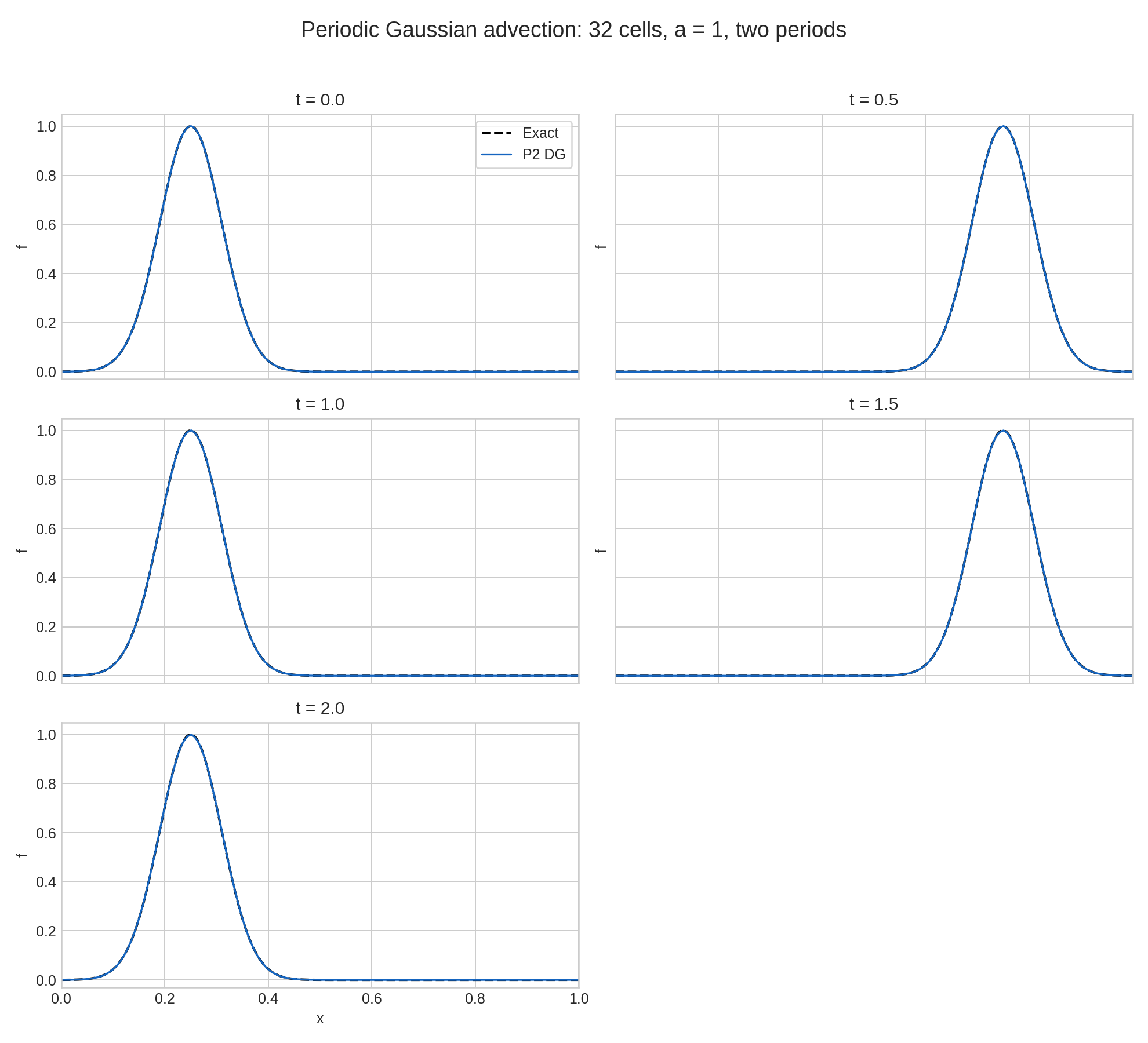
Just increasing the polynomial order to 2 dramatically improves the solution: at this resolution the DG results is essentially exact. Even at much coarser resolution, say 12 cells, the solution shows much lower diffusion and dispersion than the corresponding FV solutions.

In the next test we create a 2D advection solver:

/deepthought Create a 2D advection solver using a polynomial order 2 Discontinuous Galerkin scheme

After verifying and compiling the solver we run the cosin-hump problem defined above:

/simulate Simulate 2D advection in a flow with x-velocity -y+1/2 and y-velocity x-1/2 on a domain that is unit length in each direction, on a 32x32 grid using a polynomial order 2 DG scheme. Set diffusion to zero. Run till time of 2 pi. Use a “cosine hump” initial condition as described in https://ammar-hakim.org/sj/je/je12/je12-poisson-bracket.html#rigid-body-rotating-flow

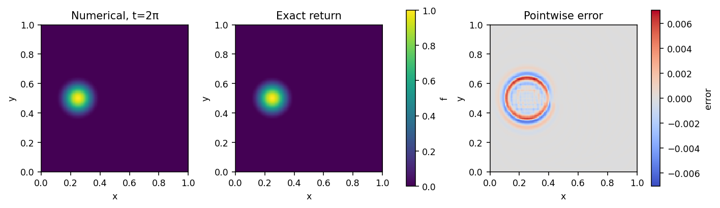
In this plot we see a dramatic improvement over the FV solution: the numerical diffusion is minimal and there is no flattening of the extrema due to limiters. Instead, and point-wise error plot shows, there is some dispersion at the edges of the profile where the gradients are largest. This is natural for DG (and also FV) schemes: as the gradient length scales get to grid size the numerical dispersion gets worse. However, in smooth regions the DG scheme performs extremely well, even when compared to a much higher resolution FV scheme.

Conclusion

In this Research Note we have discussed a fundamental equation of mathematical physics: the advection-diffusion equation. We discussed some of the properties of the equation and describe a general technique for how to derive these properties in a systematic way. Using a second-order method we solved a number of problems in 1D and 2D. All Lanyon prompts were given, with sample simulation outputs.

We should mention that for linear smooth problems the types of methods that we used above are not the best ones possible. The presence of limiters adds more diffusion than is desirable. However, these limiters are essential for discontinous solutions, for example, the square flat-top. See the No Free-Lunch Principle.

Going to higher-order methods, such as discontinuous Galerkin schemes, greatly reduces the numerical diffusion and dispersion in the solution. In fact, the DG scheme performs much better than a FV scheme even when the latter is run on a much higher grid resolution.

References and Footnotes